Yes but that means having to buffer the wiper with a non inverting amplifier. A inverting amplifier eliminates the common mode distortion problem but loads the wiper. So how do we win with this? There is a reason why you didn't use pots for tuning in your oscillator.
Yes, you are correct about the tradeoff between wiper loading and common mode distortion of a subsequent non-inverting stage. The latter, of course depends a lot on the op amp used. This is usually a bigger problem with JFET op amps. There are one or two places in my analyzer where non-inverting stages are used anyway, including the output amplifier of the oscillator. As far as I can tell, these non-inverting stages are not responsible for the distortion floor.
This tradeoff was not in my mind in using switched resistors instead of pots. I would have needed a 4-gang audio taper pot with great tracking to achieve my goal (I needed to have the oscillator and analyzer controlled by a single control and a simple linear control of frequency would be undesirable). Such a pot did not exist then, and can be hard to find today. But there are some decent such pots that might be adequate - for example some pots made for multi-channel audio systems. I would not rule out making an analyzer with a quad pot today. But I favor the use of relays.
Cheers,
Bob
Hi David, I'm interested as well. Also no hurry...If anyone is interested in the math for this attenuator. I can post a tutorial for it.
The same circuit can be set up for any taper or graduation. It will take some time to put it together so let me know.
Thanks!
Hi xavirom,
It's a coincidence that the values of those two frequencies are the same.
The resistors mentioned in table 3 are all in series. The selection of the frequency is done by changing the wiper of the rotary switch from one tie-point to another.
I tried to make that clear in my drawings.
It's a coincidence that the values of those two frequencies are the same.
The resistors mentioned in table 3 are all in series. The selection of the frequency is done by changing the wiper of the rotary switch from one tie-point to another.
I tried to make that clear in my drawings.
Hi David, I'm interested as well. Also no hurry...
Thanks!
Sure.
I was working on HP339A mods but I'll take a break from that.
I'll get started tonight.
Last edited:
Sure.
I was working on HP339A mods but I'll take a break from that.
I'll get started tonight.
Since you obviously have a THD analyzer at your disposal, what THD do you measure on the generator output pot?
Since you obviously have a THD analyzer at your disposal, what THD do you measure on the generator output pot?
Which pot?
There is trim in the oscillator feedback and a level adjust pot before the buffer IC?
Binary weighted log attenuator
This is short tutorial on how to calculate the resistor values for a binary weighted logarithmic attenuator in decibels.
The first thing to do is to choose a section constant resistance. The section constant resistance is the same as the attenuator impedance, Z. The impedance can be any practical value, 50 Ὠ, 600Ὠ, 5kὨ etc. The attenuator network requires a terminating load equal to the attenuator impedance.
The next step is to decide on the number of steps and the step size. The number of steps is two raised to the number of attenuator sections, (2NumSec ), For a eight section attenuator 20, 21 , 22 , 23, 24, 25, 26, 27 ,. The number of steps is the sum of the binary weights, 1, 2, 4, 8, 16, 32, 64, 128, which sums to 255 steps. The step size can be any decibel value, -0.5dB, -1dB, -10dB, -20dB. Each attenuator section is weighted by step size multiplied by the binary weight.
In the following design example 9.2k Ὠ is chosen for a section constant, four sections, 15 steps and a step size -1dB. The attenuator has a constant input resistance and varying output resistance. Each section is calculated separately according to the weight -1dB, -2dB, -4dB and -8dB. Each subsequent section loads the section before it and the last output is loaded by RL.
First, calculate the attenuation factor for the section weight. The attenuation factor is found by taking the antilog (10x) for x = (-dB/20).
Section 1: -1dB: 10(-1/20) = 0.89125094
Section 2: -2dB: 10(-2/20) = 0.79432823
Section 3: -4dB: 10(-4/20) = 0.63095734
Section 4: -8dB: 10(-8/20) = 0.39810717
To calculate the resistances for our attenuator we also require factors for the difference from 0dB. 0dB is a factor of 1 (unity). Theory: The range of ~Attenuation~ lies between 0 and 1. Therefore, the sum of the two factors equals 1.
Section 1 -1dB: 1 - 0.89125094 = 0.1874906
Section 2 -2dB: 1 - 0.79432823 = 0.20567177
Section 3 -4dB: 1 - 0.63095734 = 0.36904266
Section 4 -8dB: 1 - 0.39810717 = 0.60189283
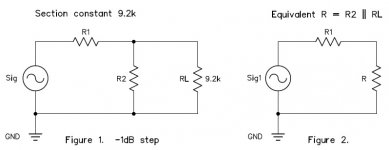
Figure 1 and figure 2 shows the voltage divider for section 1 which consists of R1, R2 and the load RL. To simplify the calculation let R = R1||RL. The values for R1 and R are calculated as follows
Section constant 9.2k Ὠ
R1 9.2k Ὠ * 0.1874906 = 1000.4914 1k Ὠ
R 9.2k Ὠ * 0.89125094 = 8199.5086 8.2 k Ὠ
R can also be found by, R = 9.2k Ὠ - 1k Ὠ = 8.2 k Ὠ
Now extract R2 from R. We will use the parallel formula for resistance. We know RL is 9.2k Ὠ, R = 8.2 k Ὠ and R1 is 1k Ὠ.
1/R = 1/R2 + 1/RL
1/8.2 k Ὠ = 1/R2 +1/9.2k Ὠ. Re arranging
1/8.2 k Ὠ - 1/9.2k Ὠ = 1/R2
R2 = 1/ (1/8.2 k Ὠ - 1/9.2k Ὠ)
R2 = 1/ 0.00001326 = 75.4k Ὠ
All other sections are calculated in the same way using the appropriate section factors.
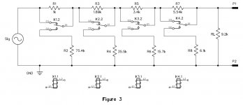
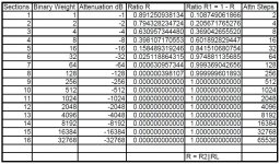
Table 1 lists factors in 1dB steps and up to 16 sections. You can see from the table 1 that it’s not really practical to do more than eight sections. Figure 3 shows the complete four section switched attenuator. Larger step attenuators can be created by simply adding on more sections and repeating the calculations. An excel spread sheet is handy for generating attenuation factors and calculating the resistances for any number of sections and step sizes.
Sections of multiple attenuators can be cascade to make a combinational attenuator. For example a four section 1dB step attenuator can be cascade with a four section 10dB step attenuator. A binary weighted attenuator can be limited to 10 steps making a decade attenuator. The binary weighted attenuator is switched in a binary count fashion.
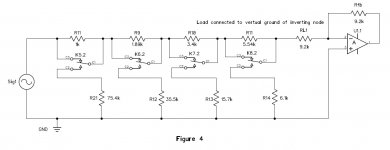
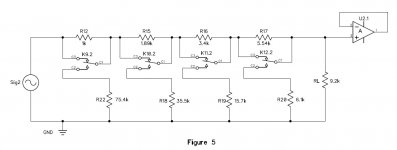
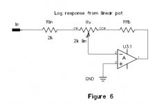
Figure 5 and 6 show how to interface the attenuator to an op amp. Figure 6 show a way of using a linear pot for a log response. A linear stepped attenuator can replace the pot..
In a second Part to this tutorial we’ll look at design ideas for controlling the binary weighted attenuator with a rotary encoder, how other tapers can be created in a similar way using the same circuit. We’ll also take a look at how this circuit can be used to tune a State Variable Oscillator.
Suggested reading: Thévenin and Norton Equivalent Circuits
This is short tutorial on how to calculate the resistor values for a binary weighted logarithmic attenuator in decibels.
The first thing to do is to choose a section constant resistance. The section constant resistance is the same as the attenuator impedance, Z. The impedance can be any practical value, 50 Ὠ, 600Ὠ, 5kὨ etc. The attenuator network requires a terminating load equal to the attenuator impedance.
The next step is to decide on the number of steps and the step size. The number of steps is two raised to the number of attenuator sections, (2NumSec ), For a eight section attenuator 20, 21 , 22 , 23, 24, 25, 26, 27 ,. The number of steps is the sum of the binary weights, 1, 2, 4, 8, 16, 32, 64, 128, which sums to 255 steps. The step size can be any decibel value, -0.5dB, -1dB, -10dB, -20dB. Each attenuator section is weighted by step size multiplied by the binary weight.
In the following design example 9.2k Ὠ is chosen for a section constant, four sections, 15 steps and a step size -1dB. The attenuator has a constant input resistance and varying output resistance. Each section is calculated separately according to the weight -1dB, -2dB, -4dB and -8dB. Each subsequent section loads the section before it and the last output is loaded by RL.
First, calculate the attenuation factor for the section weight. The attenuation factor is found by taking the antilog (10x) for x = (-dB/20).
Section 1: -1dB: 10(-1/20) = 0.89125094
Section 2: -2dB: 10(-2/20) = 0.79432823
Section 3: -4dB: 10(-4/20) = 0.63095734
Section 4: -8dB: 10(-8/20) = 0.39810717
To calculate the resistances for our attenuator we also require factors for the difference from 0dB. 0dB is a factor of 1 (unity). Theory: The range of ~Attenuation~ lies between 0 and 1. Therefore, the sum of the two factors equals 1.
Section 1 -1dB: 1 - 0.89125094 = 0.1874906
Section 2 -2dB: 1 - 0.79432823 = 0.20567177
Section 3 -4dB: 1 - 0.63095734 = 0.36904266
Section 4 -8dB: 1 - 0.39810717 = 0.60189283
Figure 1 and figure 2 shows the voltage divider for section 1 which consists of R1, R2 and the load RL. To simplify the calculation let R = R1||RL. The values for R1 and R are calculated as follows
Section constant 9.2k Ὠ
R1 9.2k Ὠ * 0.1874906 = 1000.4914 1k Ὠ
R 9.2k Ὠ * 0.89125094 = 8199.5086 8.2 k Ὠ
R can also be found by, R = 9.2k Ὠ - 1k Ὠ = 8.2 k Ὠ
Now extract R2 from R. We will use the parallel formula for resistance. We know RL is 9.2k Ὠ, R = 8.2 k Ὠ and R1 is 1k Ὠ.
1/R = 1/R2 + 1/RL
1/8.2 k Ὠ = 1/R2 +1/9.2k Ὠ. Re arranging
1/8.2 k Ὠ - 1/9.2k Ὠ = 1/R2
R2 = 1/ (1/8.2 k Ὠ - 1/9.2k Ὠ)
R2 = 1/ 0.00001326 = 75.4k Ὠ
All other sections are calculated in the same way using the appropriate section factors.
Table 1 lists factors in 1dB steps and up to 16 sections. You can see from the table 1 that it’s not really practical to do more than eight sections. Figure 3 shows the complete four section switched attenuator. Larger step attenuators can be created by simply adding on more sections and repeating the calculations. An excel spread sheet is handy for generating attenuation factors and calculating the resistances for any number of sections and step sizes.
Sections of multiple attenuators can be cascade to make a combinational attenuator. For example a four section 1dB step attenuator can be cascade with a four section 10dB step attenuator. A binary weighted attenuator can be limited to 10 steps making a decade attenuator. The binary weighted attenuator is switched in a binary count fashion.
Figure 5 and 6 show how to interface the attenuator to an op amp. Figure 6 show a way of using a linear pot for a log response. A linear stepped attenuator can replace the pot..
In a second Part to this tutorial we’ll look at design ideas for controlling the binary weighted attenuator with a rotary encoder, how other tapers can be created in a similar way using the same circuit. We’ll also take a look at how this circuit can be used to tune a State Variable Oscillator.
Suggested reading: Thévenin and Norton Equivalent Circuits
Attachments
Since you obviously have a THD analyzer at your disposal, what THD do you measure on the generator output pot?
For a "stock" HP339A thd --- see the Low Distortion Audio -Range Osc thread.
... #4322-25
THx-RNMarsh
Last edited:
we have some newer plots for input nonlinear Z distortion for some TI parts (10k input R)
http://www.diyaudio.com/forums/vendors-bazaar/283672-new-audio-op-amp-opa1622-9.html#post4636374
http://www.diyaudio.com/forums/vendors-bazaar/283672-new-audio-op-amp-opa1622-10.html#post4637092
http://www.diyaudio.com/forums/vendors-bazaar/283672-new-audio-op-amp-opa1622-9.html#post4636374
http://www.diyaudio.com/forums/vendors-bazaar/283672-new-audio-op-amp-opa1622-10.html#post4637092
This is short tutorial on how to calculate the resistor values for a binary weighted logarithmic attenuator in decibels.
The first thing to do is to choose a section constant resistance. The section constant resistance is the same as the attenuator impedance, Z. The impedance can be any practical value, 50 Ὠ, 600Ὠ, 5kὨ etc. The attenuator network requires a terminating load equal to the attenuator impedance.
The next step is to decide on the number of steps and the step size. The number of steps is two raised to the number of attenuator sections, (2NumSec ), For a eight section attenuator 20, 21 , 22 , 23, 24, 25, 26, 27 ,. The number of steps is the sum of the binary weights, 1, 2, 4, 8, 16, 32, 64, 128, which sums to 255 steps. The step size can be any decibel value, -0.5dB, -1dB, -10dB, -20dB. Each attenuator section is weighted by step size multiplied by the binary weight.
In the following design example 9.2k Ὠ is chosen for a section constant, four sections, 15 steps and a step size -1dB. The attenuator has a constant input resistance and varying output resistance. Each section is calculated separately according to the weight -1dB, -2dB, -4dB and -8dB. Each subsequent section loads the section before it and the last output is loaded by RL.
First, calculate the attenuation factor for the section weight. The attenuation factor is found by taking the antilog (10x) for x = (-dB/20).
Section 1: -1dB: 10(-1/20) = 0.89125094
Section 2: -2dB: 10(-2/20) = 0.79432823
Section 3: -4dB: 10(-4/20) = 0.63095734
Section 4: -8dB: 10(-8/20) = 0.39810717
To calculate the resistances for our attenuator we also require factors for the difference from 0dB. 0dB is a factor of 1 (unity). Theory: The range of ~Attenuation~ lies between 0 and 1. Therefore, the sum of the two factors equals 1.
Section 1 -1dB: 1 - 0.89125094 = 0.1874906
Section 2 -2dB: 1 - 0.79432823 = 0.20567177
Section 3 -4dB: 1 - 0.63095734 = 0.36904266
Section 4 -8dB: 1 - 0.39810717 = 0.60189283
Figure 1 and figure 2 shows the voltage divider for section 1 which consists of R1, R2 and the load RL. To simplify the calculation let R = R1||RL. The values for R1 and R are calculated as follows
Section constant 9.2k Ὠ
R1 9.2k Ὠ * 0.1874906 = 1000.4914 1k Ὠ
R 9.2k Ὠ * 0.89125094 = 8199.5086 8.2 k Ὠ
R can also be found by, R = 9.2k Ὠ - 1k Ὠ = 8.2 k Ὠ
Now extract R2 from R. We will use the parallel formula for resistance. We know RL is 9.2k Ὠ, R = 8.2 k Ὠ and R1 is 1k Ὠ.
1/R = 1/R2 + 1/RL
1/8.2 k Ὠ = 1/R2 +1/9.2k Ὠ. Re arranging
1/8.2 k Ὠ - 1/9.2k Ὠ = 1/R2
R2 = 1/ (1/8.2 k Ὠ - 1/9.2k Ὠ)
R2 = 1/ 0.00001326 = 75.4k Ὠ
All other sections are calculated in the same way using the appropriate section factors.
Table 1 lists factors in 1dB steps and up to 16 sections. You can see from the table 1 that it’s not really practical to do more than eight sections. Figure 3 shows the complete four section switched attenuator. Larger step attenuators can be created by simply adding on more sections and repeating the calculations. An excel spread sheet is handy for generating attenuation factors and calculating the resistances for any number of sections and step sizes.
Sections of multiple attenuators can be cascade to make a combinational attenuator. For example a four section 1dB step attenuator can be cascade with a four section 10dB step attenuator. A binary weighted attenuator can be limited to 10 steps making a decade attenuator. The binary weighted attenuator is switched in a binary count fashion.
Figure 5 and 6 show how to interface the attenuator to an op amp. Figure 6 show a way of using a linear pot for a log response. A linear stepped attenuator can replace the pot..
In a second Part to this tutorial we’ll look at design ideas for controlling the binary weighted attenuator with a rotary encoder, how other tapers can be created in a similar way using the same circuit. We’ll also take a look at how this circuit can be used to tune a State Variable Oscillator.
Suggested reading: Thévenin and Norton Equivalent Circuits
Hi David,
VERY nice piece of work! Maybe you should publish it as an article in AX or Elektor.
BTW, the pot arrangement you showed is what I would have used in a lower-cost version of my THD analyzer for continuous frequency control.
Cheers,
Bob
This is short tutorial on how to calculate the resistor values for a binary weighted logarithmic attenuator in decibels.
Hi Davada,
Thank you for this detailed and clear tutorial. I'm gonna read and digest it in parts.
")
Looking forward to the next chapter. But again, no hurry.
Best regards, Rob.
Which pot?
There is trim in the oscillator feedback and a level adjust pot before the buffer IC?
The pot that adjust oscillator output level is the one that corresponds the most to a typical audio usages, so that is the natural one to test. Also - testing should be obvious and easy. Loop the oscillator output to the input of the THD analyzer, and test.
Internal adjust pots may be completely out of the signal path or partially isolated from it.
Hi David,
VERY nice piece of work! Maybe you should publish it as an article in AX or Elektor.
Bob
I agree, that would be a terrific article. David, I have contact info if you need it (hint,hint
).Hi David,
VERY nice piece of work! Maybe you should publish it as an article in AX or Elektor.
... or in Linear Audio.
Jan
For a "stock" HP339A thd --- see the Low Distortion Audio -Range Osc thread.
... #4322-25
To be relevant and helpful:
http://www.diyaudio.com/forums/equipment-tools/205304-low-distortion-audio-range-oscillator-433.html#post4603528
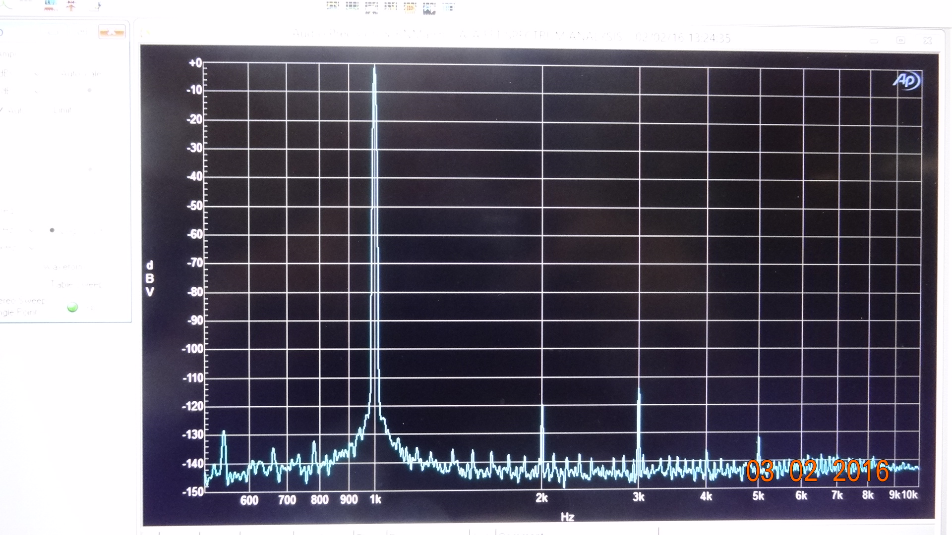
If we made a wild unfounded assumption and said that *all* of the THD at the output of the HP 339 was due to the output level potentiometer, we are still talking >115 dB down. That is very inaudible,
and even not all that easy to measure with modern test gear.
IME even some pretty cheap commodity pots from China are better than that. I'm talking < $1 on eBay.
The counterpoint is that all sorts of common audio components can but might not have as much or far more nonlinear distortion, and that includes a commonly recommended alternative, relays. Plugs, jacks, edge connectors, fixed resistors, capacitors used wrong, not to mention tubes, transistors, ICs and opto-isolators can be far worse than a good cheap pot in good condition.
Furthermore, if we are talking THD+N, then even an ideal voltage divider will significantly increase the measured residual.
Last edited:
Hi David,
VERY nice piece of work! Maybe you should publish it as an article in AX or Elektor.
BTW, the pot arrangement you showed is what I would have used in a lower-cost version of my THD analyzer for continuous frequency control.
Cheers,
Bob
Thanks Bob.
That's a big compliment since this is the first bit of writing I've done for a public forum.
I didn't think about publishing it.
I used the pot arrangement in a continuously tuned oscillator using an XR2206.
I got hired on at Vancouver's Science World 8 weeks before official opening to help them finish their exhibits and the oscillator was one of them. It was a short employment but I got to do some neat things.
Section 1 -1dB: 1 - 0.89125094 = 0.1874906
Section 2 -2dB: 1 - 0.79432823 = 0.20567177
Section 3 -4dB: 1 - 0.63095734 = 0.36904266
Section 4 -8dB: 1 - 0.39810717 = 0.60189283
Figure 1 and figure 2 shows the voltage divider for section 1 which consists of R1, R2 and the load RL. To simplify the calculation let R = R1||RL. The values for R1 and R are calculated as follows
Section constant 9.2k Ὠ
R1 9.2k Ὠ * 0.1874906 = 1000.4914 1k Ὠ
R 9.2k Ὠ * 0.89125094 = 8199.5086 8.2 k Ὠ
Hi David,
I detected a small typo, better to correct that before publishing it in a famous magazine
Section 1 -1dB: 1 - 0.89125094 = 0.10874906
Section 2 -2dB: 1 - 0.79432823 = 0.20567177
Section 3 -4dB: 1 - 0.63095734 = 0.36904266
Section 4 -8dB: 1 - 0.39810717 = 0.60189283
Figure 1 and figure 2 shows the voltage divider for section 1 which consists of R1, R2 and the load RL. To simplify the calculation let R = R1||RL. The values for R1 and R are calculated as follows
Section constant 9.2k Ὠ
R1 9.2k Ὠ * 0.10874906 = 1000.4914 1k Ὠ
R 9.2k Ὠ * 0.89125094 = 8199.5086 8.2 k Ὠ
- Status
- This old topic is closed. If you want to reopen this topic, contact a moderator using the "Report Post" button.
- Home
- Design & Build
- Equipment & Tools
- Another realization of Bob Cordell's THD Analyzer