I would say the simulations look reasonable given the pure sine nature. Most polars are shown 1/3 octave which washes away a lot of problems (most of them actually). I use critical band smoothing which is about 1/20th octave above 1 kHz. This is still going to smooth out things that you will see with a simulation at a fixed frequency. All in all I would say that your sims - when properly considered - show precisely what the issues are. When taken out of context they can show whatever the poster wants them to show. Its important that people see both sides.
Thanks Earl.
By the way I tried your website but I could not load it. Do you show polar maps for the OSWG. Those are what I know best and could tell if the sims reflect reality or not.
I'm not sure what that could be. The site is up, although it can be slow some times. Have you tried different browsers or security settings?
I show polar maps for all the horns and waveguides I have simulated. Last time you looked at it, you commented that one of the simulations was very close to the performance of a small waveguide.
I would have no issue with giving you the dimension of one of my waveguides. I don't remember you asking. I have a ton of very accurate data on them that could be used to validate a model.
I asked back here, but you replied "As to running simulations on my waveguides, that seems unnecessary. I mean simulations are great when you don't have the actual device or you want to know about changes, but if you actually have the device then simulations are not really of much interest." But if you want to send me them (PM?), I could easily run a simulation on that configuration. Another validation would be nice.
I plan to take my measurements up one more notch to better quantify the performance. My hope is that with the next installment I can begin to sort out the HOMs. It's clear that something like that is occurring in your sims as the angular features are not at all constant - a key feature of HOMs. The question that is very hard to sort out is what are caused by the mouth and what are from down into the device. No far field measurement could ever sort that out.
Wouldn't a mode based simulation also be able to give you that kind of information? While working on modal model using a stepped cylindrical approximation, I played with tracing the amplitudes of the pressure and velocity modes throughout the horn.
Are you aware that I can reconstruct the velocity at the mouth by a reverse (ala holographic) technique from measured data. It works down to about a 1/2 wavelength now because the boundary conditions are not precise. My plan is to use a large flat baffle which should allow for about a 1/4 wavelength resolution and then possible a reconstruction of the waves inside the device from that. A lot of work but the only way to get to the nitty-gritty of these things.
Yes, you write about that technique in your book, right? It looks very interesting. I would love to have something like that working here at the University too, because it would be interesting to look at the AH425 and other horns that way.
Will you decompose the mouth velocity into cylindrical modes, or OS or spherical modes?
-Bjørn
Bjorn
It is all modal, but when you mention using cylindrical that implies an analytical model and what I am doing is reverse engineering an actual device from measurements. (As we discussed, I would use conical section instead of cylindrical.) I have already shown the existence of HOMs theoretically so that's not necessary, but real devices are not exactly what we analyze and I want to measure details like what the compression driver and the mouth flare contribute. Those things are very difficult to analyze theoretically.
The current measurement scheme uses spherical radiation modes and then calculates what the velocities would be on a sphere, a section of which is located where the mouth is. But this boundary condition is not exactly correct (the box is square not round).
It is also possible to use the modes for a piston in a baffle - I think that this is described in my book. With a horn placed in a large baffle (> 1/2 wavelength at the lowest frequency of interest) this boundary is very close to the real thing and so the reconstruction should be quite accurate.
This would give me an accurate shape of the wave front at the mouth. Using the OS modes defined at the mouth, one could calculate each modes contribution to that velocity distribution. The problem that I am wrestling with is how to account for the mouth diffraction. If I can get that resolved then I'm home free.
An extremely precise measurement would use an actual sphere around the horns mouth. This would be so exact that even the mouth diffraction could be calculated. But making a sphere that large would be a task. A large baffle is not so bad - just a piece of MDF with a hole in it.
So if I gave you the dimensions of my largest waveguide you could simulate that in a flat baffle? I could then measure this same configuration and compare. I'd be willing to do that. How do you account for the drivers non-flat velocity characteristics?
When I finished the Ariels in 1993, I listened at first on my trusty Audionics CC-2, which is still one of the better transistor amps out there. I also know what's inside the amplifier, since Bob Sickler, the designer, walked me through the circuit as he designed it.
Since the Ariel was, after all, designed for DHT-triode amplifiers, I listened to a whole bunch, as well as antiques like the Dyna Stereo 70. To my dismay, the amps all sounded different, and this applied to the transistor amps as well. None sounded alike.
This wasn't true on my previous speaker, the LO-2, which was my last project at Audionics in 1979. The LO-2 was a linear-phase minimonitor-style speaker, but only had an efficiency of 86 dB/meter. The Ariel is a genuine 92 dB/meter.
Well, that made a difference. A big difference. More than I expected. Now I could hear easily hear differences between amplifiers, despite the Ariel being a pretty benign load (conjugate network in the crossover, transmission-line LF loading, etc.).
…
Hi Lynn,
This may not be unique to Ariel.
No two amplifiers, SS or tubes, sounded the same on my setup, with both my previous speakers and present one.
Possibly, the Ariels are more revealing than other speakers, I haven’t heard them.
Jean-Michel,Hello,
You are forgetting that the simulation of the AH424 is based on a theorical source having a constant velocity.
Real measuremenst made on axisymetrical Le CLéac'h horns, never show an increasing slope of the on-axis frequency response curve.
See as an example a real measurement :
Horns
And no JMLC horn sounds overly bright !
Best regards from Paris, France
Jean-Michel Le Cléac'h
No forgetting happened, I made the mistaken assumption the four of Bjørn's charts I re-posted were measured response, not all simulations.
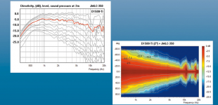
Thanks for linking a real measurement, clearly the JMLC-350 is relatively flat on axis, with a -6 dB beamwidth from around 100 degrees at 800 to 20 degrees at 8000 Hz, a five to one variance over the decade.
As you point out, it would not sound overly bright on axis, though it would sound dull by comparison off axis.
What does the red line in the "Directivity,(dB),level,sound pressure at 2m" chart refer to?
What are the off axis angles in that chart?
Are the fluctuations in beamwidth above 8000 Hz driver type and exit size or horn related or both?
Do you have the measured response of the JMLC-350 with a 1" exit driver?
Do you think the AH425 horn Lynn uses would have similar dispersion to the JMLC-350 ?
Art
Attachments
Last edited:
And hence the value of LEDEThe only way that this is possible is for the room to be completely dead - an anechoic chamber. Otherwise the small room queues will always dominate because they are shorter (longer is never a problem.) But then this leaves a completely lifeless local acoustic and only music with a lot of venue acoustic will sound even remotely correct - but then the acoustic is still coming from the wrong place. So this approach simply kills the kind of music that I prefer and that is simply 2 channel studio work. So a dead local acoustic is simply not an option for me. I make the local acoustic as live as possible.
Rock concerts don't have any venue acoustic since the feed is generally taken directly from the performers and not the room. Played loud enough, the local acoustic kind of goes away and the playback realism becomes quite convincing. Its gone at lower levels, probably because the expectation is for loud.
It is also possible to use the modes for a piston in a baffle - I think that this is described in my book. With a horn placed in a large baffle (> 1/2 wavelength at the lowest frequency of interest) this boundary is very close to the real thing and so the reconstruction should be quite accurate.
Yes, the radiation from a non-ridgid piston, i.e. with a given velocity distribution, mounted in a baffle, is described in your book. You also have some suggestions for a measuring method to find the mode amplitudes for that velocity distribution, expressed in cyldindrical coordinates.
So if I gave you the dimensions of my largest waveguide you could simulate that in a flat baffle? I could then measure this same configuration and compare. I'd be willing to do that. How do you account for the drivers non-flat velocity characteristics?
I can simulate the waveguide mounted in an infinite baffle using the BERIMA BEM/Rayleigh Integral Method. Then I get the mouth velocity directly as well. By giving the elements at the throat different velocities, many different velocity profiles could be built up. The channel inside the compression driver could also be included in the simulation, but changing the throat velocity profile is faster (the whole surface integration does not need to be recalculated, although to do this would require some modification to the way the boundary conditions are set up in the SW. No big deal, I think).
I can also simulate the waveguide mounted in a round finite baffle, if that is of any interest to you.
Usually I generate the horn contours parametrically, so for the OS, I would need throat diameter and tangent angle (if different from zero), the length of the OS section and the mouth diameter, and the radius and final angle of the mouth flare. I think that should suffice to create the boundary.
Regards,
Bjørn
A finite baffle compared to an infinite baffle would be a very interesting test. That would tell me what kinds of errors using a finite baffle would make in the infinite baffle calculations.
Basically you could do this: Find the mouth velocities for a flat plane throat source, then for a first cylindrical mode, then for a second, etc. In that way you would know the mouth velocities for a range of orthogonal throat velocities. That would solve the whole problem right there I think.
We should talk off-line because I doubt many others are following this. I am not sure that I have your E-mail. I'll check.
But my question above was more along the lines of how do you account for using a real driver when comparing simulated data to measured data?
Earl,A finite baffle compared to an infinite baffle would be a very interesting test. That would tell me what kinds of errors using a finite baffle would make in the infinite baffle calculations.
But my question above was more along the lines of how do you account for using a real driver when comparing simulated data to measured data?
I would also be interested in the answer to that question, comparing simulations and measured response is similar to comparing apples to oranges.
Art
That set me to wondering what size room and what sort of speaker placement could get you to >10 ms for 1st reflections. That's only about 11 feet (343 cm) of difference.I would guess that a significant transition would occur once you could push the earliest reflections beyond 10 ms. Things would start to change significantly once that happened.
Doing simulations of several rooms, it appears that the big rooms have an interesting advantage over the small ones. By the time the wave gets to the listener, it is already very homogeneous in a large room. Not so in a small room, even with good speaker placement. The reflections in a large room are less distinct, the major reflections may be swamped by a myriad of small ones. In a small room the reflection can be more distinct, separated from each other by relative silence.
Happy Thanksgiving, everyone!
I can't do the math to follow along with my own programming and share results, but I was certainly following that discussion with interest, so just a different thread would be cool, I think.We should talk off-line because I doubt many others are following this.
I am sure a very significant amount of effort is necessary to develop a math model or simulation with precision. There can even be lots of differences between different existing software and methods, and is why you have different magnitudes of software.
There is a lot of truth in what you say. The danger occurs when the arguments fall into mathematical models where they are subtly flawed or are a compromise. This applies when not all the variables are factored in.
Anything we do from a pure point source or a pure planar source is frought with very complex problems It inevitably means some loss of aural data in differing possible ways. There are too many compromises being juggled in the air. I guess the OS Lecleach issue sounds the most interesting and it may be the next step forward with the best CD's
Clearly their is more work to do. The more CSD's impulse tests the more apparent what the researchers are grappling with. HOM seems the most persistent but not the only problem from the CSD and step tests
Last edited:
That set me to wondering what size room and what sort of speaker placement could get you to >10 ms for 1st reflections. That's only about 11 feet (343 cm) of difference.
Doing simulations of several rooms, it appears that the big rooms have an interesting advantage over the small ones. By the time the wave gets to the listener, it is already very homogeneous in a large room. Not so in a small room, even with good speaker placement. The reflections in a large room are less distinct, the major reflections may be swamped by a myriad of small ones. In a small room the reflection can be more distinct, separated from each other by relative silence.
Happy Thanksgiving, everyone!
And to tie this to Dr. Geddes's approach--
while the strength and diffusiveness of reflections could be addressed to some extent with room treatments, the timing can't. The hallmark of room size is the ITDG (Initial time delay gap- the period before any room effect information is received) followed by the density and direction of first reflections (which also tells us the character of the room).
Earl's answer of [high directivity + speaker orientation + live walls] to intentionally generate (relatively) later reflections while reducing the earliest reflections is the only passive 2-channel solution that mostly 'works' to virtually enlarge a room. Get the the brain to identify the later, denser, more diffuse package of reflections as if they are the first reflections, and voila, bigger room.
Last edited:
I use a similar approach, but I tend to like the effect of diffusion better than absorption. A room does need both, for sure. I wonder if judicious use of diffusion would imitate the sound field of a larger room? Back to the text books!
Diffusion can't really simulate a larger room, just make one less obviously small, if that makes sense. There is a ton of confusion in the application of the terms diffuse (a condition), diffusion (an action), and diffusor (a device).
Although rarely stated so clearly (thank you, Marketing), The true purpose of diffusion in small rooms is simply to reduce the small room 'signature' without excessive absorption.
Ironically, The best way to simulate larger room is with some later Temporally Preserved "TPR" Reflections. These are ones that still have phase information for the original signal - planar reflections.
Read that twice, because nobody ever says it!
By design, Diffusion devices actually destroy phase information. I'm not saying this is bad, but the simple fact is that planar reflections are only beneficial if they are many and adequately delayed. As you pointed out above, this is the opposite of what occurs in small rooms: discrete and spaced early reflections.
Interestingly, the best rated concert halls contain some scattering and many planar reflections, and nothing that would technically be called a diffusor!
Diffusion is essential for recording studios, as the source and listener (microphone) positions could be anywhere. In a playback room, where the source location is fixed, diffusion could be moot or even undesirable IF one is able to achieve the conditions that Doc Geddes prescribes.
Setups that are non-symmetrical, etc usually need treatment intervention, IMHO.
--Mark
Thanks Mark, good info.
Well that's what I try to do with them. Break up the distinct reflections without killing the ambiance too much. Diffusers are much more labor intensive to build than absorbers.Thetrue purpose of diffusion in small rooms is simply to reduce the small room 'signature' without excessive absorption.
Both the change when using a finite baffle compared to an infinite one, and what the radiated field looks like for different cylindrical modes would both be very interesting. Should be fairly easy to implement.
Just send me a PM if you can't find it.
Right. Well, I'm not sure. Simulating the driver using the standart lumped parameter model is too simple for such a comparison, I think. And if the acoustic paths in the driver were to be simulated in BEM, it would be difficult to get all dimensions right. In addition comes the fact that viscous losses would not be included, and the mechanical part, with breakups etc could not be simulated.
If it was possible to measure the pressure near the throat surface, that could be used as a reference that all measurements could be normalized to. For instance, the pressure could be measured at the waveguide wall, and the pressure at the same point could be computed in the simulation. The measured pressure in this point could be used to normalize the measurements, and the simulated pressure to normalize the simulations.
Alternatively, Makarski shows how to measure the T-matrix of the driver, but that may be to big a job if you are only interested in the behaviour of the waveguide.
Regards,
Bjørn
We should talk off-line because I doubt many others are following this. I am not sure that I have your E-mail. I'll check.
Just send me a PM if you can't find it.
But my question above was more along the lines of how do you account for using a real driver when comparing simulated data to measured data?
Right. Well, I'm not sure. Simulating the driver using the standart lumped parameter model is too simple for such a comparison, I think. And if the acoustic paths in the driver were to be simulated in BEM, it would be difficult to get all dimensions right. In addition comes the fact that viscous losses would not be included, and the mechanical part, with breakups etc could not be simulated.
If it was possible to measure the pressure near the throat surface, that could be used as a reference that all measurements could be normalized to. For instance, the pressure could be measured at the waveguide wall, and the pressure at the same point could be computed in the simulation. The measured pressure in this point could be used to normalize the measurements, and the simulated pressure to normalize the simulations.
Alternatively, Makarski shows how to measure the T-matrix of the driver, but that may be to big a job if you are only interested in the behaviour of the waveguide.
Regards,
Bjørn
Earl,
I would also be interested in the answer to that question, comparing simulations and measured response is similar to comparing apples to oranges.
Art
Hi Art
I have spent my life between the measurement world and the simulation one. They may be "apples to oranges", but they don't have to be. there are very good uses for both and when the two come together then you know that you really understand the situation. The exact same is true about measurements and perception. Only when the two come together can you say with any certainty that you understand what is going on.
When people say that there are things that they hear that cannot be measured, it's a clear indication that they don't understand something, because if they did then this could not be true.
So the answer is you have to do it all, utilizing each in that domain for which it is best suited; analysis for early development when you don't have anything to measure; measurements for when you have a prototype; and psychoacoustics for when you are refining the prototype. If you know what you are doing this will always result in a success - its science not magic.
I am interested in this conversation as well. I always enjoy learning!
That's fine, but I feel guilty hijacking this thread. Perhaps it should be continued elsewhere.
- Home
- Loudspeakers
- Multi-Way
- Beyond the Ariel